gamRTMB

Distributional (GAMLSS-style) regression where smooth terms can enter every parameter of a distribution, not just the mean.

The package is mostly glue, by design:

• mgcv builds the bases and penalties, and mgcv::smooth2random() reparameterises the penalized coefficients as iid Gaussian random effects — except where the penalty is already a sparse precision matrix, which keeps it and uses RTMB::dgmrf() instead;
• RTMB supplies automatic differentiation and the Laplace approximation;
• RTMBdist supplies the log-densities, each in its own native parameterisation — a skew normal is modelled as xi, omega, alpha, not as generic location/scale/shape.

Restricted maximum likelihood is the default, effective degrees of freedom per smooth agree with mgcv, and smoothing parameters can be shared between terms and between distributional parameters.

Installation

# install.packages("pak")
pak::pak("janolefi/gamRTMB")

Example

MASS::mcycle measures head acceleration in a simulated motorcycle crash. The mean is famously hard to model — and the variance changes just as much.

library(gamRTMB)
data(mcycle, package = "MASS")

fit <- gamRTMB(accel ~ list(mean = ~ s(times, k = 20),
                            sd   = ~ s(times, k = 10)),
               data = mcycle)
summary(fit)
#> 
#> Family: norm   [dnorm from RTMB]
#> Links:  mean = identity,  sd = log
#> 
#> Formula:
#>   mean ~ s(times, k = 20)
#>     sd ~ s(times, k = 10)
#> 
#> Parametric coefficients:
#>                   Estimate Std. Error z value Pr(>|z|)    
#> mean:(Intercept) -25.21806    1.85310  -13.61   <2e-16 ***
#> sd:(Intercept)     2.58334    0.06443   40.10   <2e-16 ***
#> ---
#> Signif. codes:  0 '***' 0.001 '**' 0.01 '*' 0.05 '.' 0.1 ' ' 1
#> 
#> Smooth terms:
#>           term    edf  k        sp
#>  mean:s(times) 14.382 19 2.893e-06
#>  sd:s(times)    7.150  9  0.009119
#> 
#> Total EDF = 23.53   n = 133
#> -REML = 587.275   logLik = -532.303   AIC = 1111.67

Once every parameter varies, the useful output is covariate-dependent quantiles rather than a mean and one standard error:

plot(fit, type = "quantile")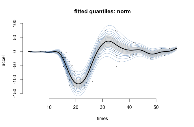

Term plots, a worm plot of randomised quantile residuals, and everything else are in vignette("gamRTMB").

What it does

Families	85, from RTMBdist plus the standard R densities; families() lists them, fam() builds one
Formula	y ~ list(mean = ~ s(x), sd = ~ s(z)), one one-sided formula per parameter, missing ones get ~1
Smooths	s(), t2(), by=, bs="fs", bs="re", shrinkage bases, and id= to share smoothing parameters
Spatial	bs="mrf" Markov random fields over an adjacency graph, or any precision matrix via xt=list(penalty=); bs="spde" Matern fields on an fmesher mesh. Both kept sparse, so a few thousand regions or mesh nodes is routine
Criterion	REML by default (coefficients integrated out by the same Laplace approximation), or ML
Inference	summary(), vcov(), edf(), AIC()/BIC(), predict() with standard errors
Diagnostics	residuals() gives randomised quantile residuals; plot(type = "worm")
Also	weights, offset() inside a parameter’s formula, na.action

Status

Early but checked. EDF and fitted values agree with mgcv::gam(family = gaulss()) to three decimals, with and without shared smoothing parameters; predict() on the fitting data reproduces the in-sample linear predictors to machine precision; and quantile standard errors match both an analytic special case and simulation from the joint posterior. The sparse GMRF route is a reparameterisation rather than an approximation, and is checked against the dense one: log-likelihood, EDF, AIC, fitted values, predictions and their standard errors all agree, on Markov random fields and on ordinary smooths alike. The SPDE precision matches the closed form $\tau^2(\kappa^4 C + 2\kappa^2 G_1 + G_2)$ to 5e-16, and the fitted range and marginal standard deviation approach their true values as the sample grows.

Not supported: te() (mgcv itself declines smooth2random(type = 2) for it — use t2()), fx = TRUE, and smooths whose unpenalized null spaces overlap (use a shrinkage basis, bs = "ts"). Not yet implemented: smooth-term p-values, 2-D smooth plots, and an extended Fellner–Schall fitting engine as an alternative to the Laplace one — dev/NOTES-fellner-schall.md records the derivation and the seams it needs.