Introduction to gamRTMB

A regression model usually lets the mean depend on covariates and treats everything else about the distribution as constant. That is often wrong, and when it is, the mean is not the part that misleads you: the intervals are.

gamRTMB fits models where every parameter of a distribution can carry smooth terms. It is mostly glue — mgcv builds the bases and penalties, RTMB supplies automatic differentiation and the Laplace approximation, and RTMBdist supplies the log-densities — so the interfaces should feel familiar if you have used either.

library(gamRTMB)

The data

MASS::mcycle records head acceleration in a simulated motorcycle crash: 133 measurements of accel against times, in milliseconds after impact. It is the standard example of a mean that is hard to model, and it also has an obvious second feature.

data(mcycle, package = "MASS")
plot(accel ~ times, data = mcycle, pch = 20, col = "grey30", bty = "n",
     xlab = "time (ms)", ylab = "acceleration (g)")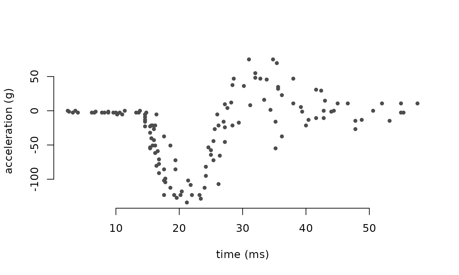

Before about 15 ms nothing happens and the points sit tightly on a flat line. Through the impact they swing violently and scatter widely, then settle. So the variance changes with time as clearly as the mean does. A model that assumes constant variance will report intervals that are far too wide early on and too narrow at the impact.

A first fit

The formula gives the response on the left and a list() of one-sided formulas on the right, one per distributional parameter. Parameters are named as the density names them, so a Gaussian is mean and sd rather than generic labels:

fam("norm")
#> gamRTMB family: norm  [dnorm, RTMB]
#>   modelled: mean (identity), sd (log)
#>   support:  continuous

Let the mean and the standard deviation each have their own smooth:

fit <- gamRTMB(accel ~ list(mean = ~ s(times, k = 20),
                            sd   = ~ s(times, k = 12)),
               data = mcycle)
fit
#> gamRTMB fit
#>   family:    norm (mean/identity, sd/log)
#>   criterion: REML   engine: laplace
#>   converged: TRUE   -REML: 587.0647   max|grad|: 2.55e-05
#>   observations: 133
#>   coefficients: 4 fixed (incl. null spaces), 28 penalized; 2 smoothing parameters

summary(fit)
#> 
#> Family: norm   [dnorm from RTMB]
#> Links:  mean = identity,  sd = log
#> 
#> Formula:
#>   mean ~ s(times, k = 20)
#>     sd ~ s(times, k = 12)
#> 
#> Parametric coefficients:
#>                   Estimate Std. Error z value Pr(>|z|)    
#> mean:(Intercept) -25.20458    1.83426  -13.74   <2e-16 ***
#> sd:(Intercept)     2.57458    0.06542   39.36   <2e-16 ***
#> ---
#> Signif. codes:  0 '***' 0.001 '**' 0.01 '*' 0.05 '.' 0.1 ' ' 1
#> 
#> Smooth terms:
#>           term    edf  k        sp
#>  mean:s(times) 14.433 19 2.869e-06
#>  sd:s(times)    7.578 11  0.008296
#> 
#> Total EDF = 24.01   n = 133
#> -REML = 587.065   logLik = -531.138   AIC = 1110.30

Both smooths are strongly non-linear: 14.4 and 7.6 effective degrees of freedom out of the 19 and 11 the bases allow. The smoothing parameters and EDFs come from a REML fit and agree with mgcv to three decimals on models both packages can express.

par(mfrow = c(1, 2))
plot(fit)

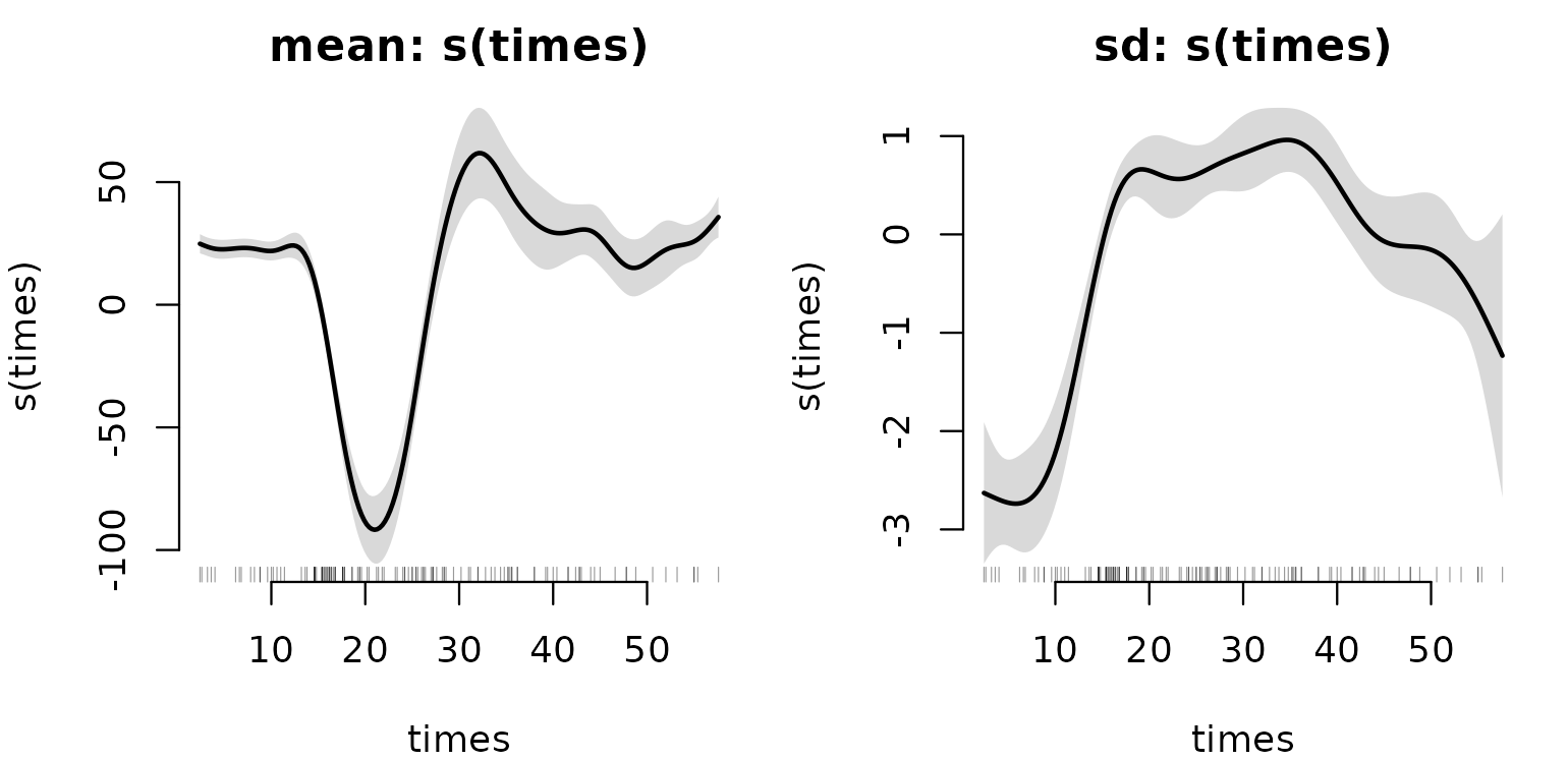
The right-hand panel is the point. The smooth on sd spans about 3.7 units on the log scale, so the fitted standard deviation varies by a factor of roughly 40 between the quiet stretch before impact and the violent part.

Was constant variance really inadequate?

Fit the same mean structure with a constant sd and compare. AIC() uses the log-likelihood at the fitted coefficients with the total effective degrees of freedom, the same convention mgcv and GAMLSS’s GAIC use, so the two are comparable:

fit0 <- gamRTMB(accel ~ list(mean = ~ s(times, k = 20), sd = ~ 1),
                data = mcycle)
c(constant_sd = AIC(fit0), smooth_sd = AIC(fit))
#> constant_sd   smooth_sd 
#>    1221.532    1110.299

A difference of that size is not a close call.

Checking the distribution, not just the mean

Randomised quantile residuals turn the whole distributional assumption into something you can look at: if the model is right they are standard normal. The worm plot is the detrended QQ plot, which makes it easier to see where a distribution is wrong.

par(mfrow = c(1, 2))
set.seed(1)
plot(fit0, type = "worm", main = "constant sd")
plot(fit,  type = "worm", main = "smooth sd")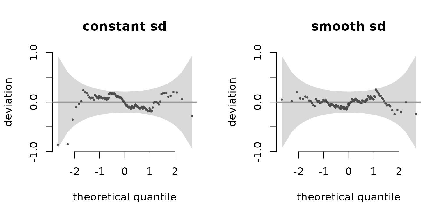

The difference is real but not dramatic: with sd held constant a few points in the lower tail leave the band, reaching about 1.4 times its width, while with a smooth sd nothing leaves it at all. Worth noting how much weaker this evidence is than the AIC gap of 111 — with 133 observations a worm plot is a blunt instrument, and it is the more useful of the two for telling you where a fit is wrong rather than whether.

Is a Gaussian the right shape at all?

With sd free the residuals look fine, but it is worth asking whether the shape needs changing too. Switching family is one argument: fam() derives the parameter names, links and starting values from any suitable density, so nothing has to be written per distribution.

A power exponential has a third parameter nu controlling the tails, with nu = 2 being exactly Gaussian:

fam("powerexp2")
#> gamRTMB family: powerexp2  [dpowerexp2, RTMBdist]
#>   modelled: mu (identity), sigma (log), nu (log)
#>   support:  continuous

fit_pe <- gamRTMB(accel ~ list(mu = ~ s(times, k = 20),
                               sigma = ~ s(times, k = 12),
                               nu = ~ 1),
                  family = fam("powerexp2"), data = mcycle)
c(nu = exp(coef(fit_pe)$beta[["nu:(Intercept)"]]))
#>      nu 
#> 41.1903
c(gaussian = AIC(fit), power_exponential = AIC(fit_pe))
#> Warning: the effective degrees of freedom are not defined at these values: 28
#> of 33 coefficients fall outside [0, 1], so the data Hessian is not positive
#> semi-definite here and H^-1 H_data is not a projection. They are reported as
#> NA. This fit has not converged -- check `max_grad`; see ?gamRTMB for the
#> starting-value and basis options.
#>          gaussian power_exponential 
#>          1110.299                NA

nu comes out near 3.7 rather than 2, which points to slightly lighter tails than Gaussian, but AIC does not prefer the richer model. So there is no case for changing the shape once the variance is free to vary. That is a useful negative result, and the interesting part is the order in which you find it: fitted with constant variance, the residuals of this data look heavy-tailed and would tempt you towards a t distribution. The tails were never the problem — the variance was.

Not every family will fit this data. Several heavier-tailed ones fail to converge here, and gamRTMB says so plainly rather than returning a fit that looks fine:

fit_t <- gamRTMB(accel ~ list(mu = ~ s(times, k = 20),
                              sigma = ~ s(times, k = 12), df = ~ 1),
                 family = fam("t2"), data = mcycle)
fit_t$convergence
#> [1] FALSE

What the model is for

Once every parameter varies, the useful output is not a mean and a single standard error but covariate-dependent quantiles:

plot(fit, type = "quantile", prob = c(0.05, 0.25, 0.5, 0.75, 0.95))

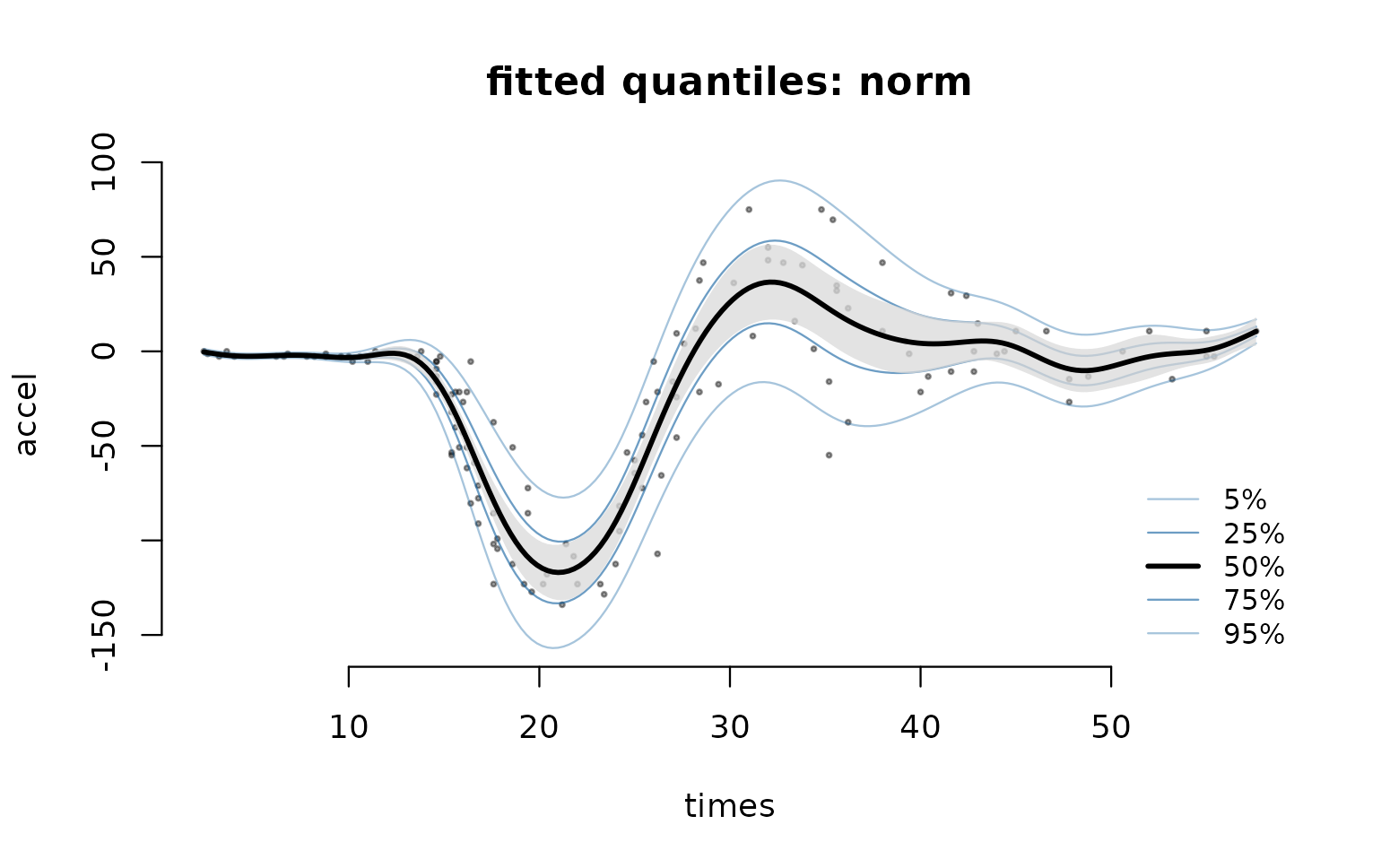
The curves contract and fan out with the fitted spread, which is exactly what the second smooth bought. The shaded band is the median curve’s own estimation uncertainty — not a prediction interval; the outer quantiles are that.

The fan summarises the fitted distribution by its quantiles. To see the shape itself, type = "density" draws the fitted density turned on its side at a few times. This works for every family, including the many that have no quantile function:

plot(fit, type = "density")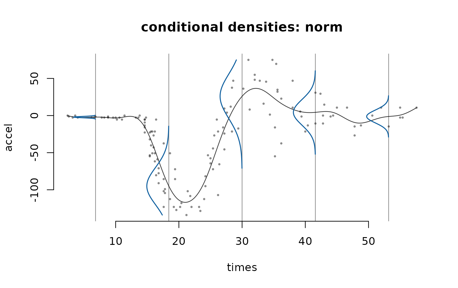

predict() gives the quantiles as numbers, with standard errors from the delta method across all the linear predictors at once:

nd <- data.frame(times = c(10, 20, 30, 40))
q <- predict(fit, newdata = nd, type = "quantile", prob = c(0.1, 0.5, 0.9),
             se.fit = TRUE)
round(cbind(times = nd$times, q$fit), 1)
#>      times   q0.1   q0.5  q0.9
#> [1,]    10   -5.1   -3.3  -1.5
#> [2,]    20 -146.0 -113.9 -81.7
#> [3,]    30  -12.3   26.0  64.3
#> [4,]    40  -24.1    4.3  32.6
round(q$se.fit, 2)
#>       q0.1 q0.5  q0.9
#> [1,]  0.77 0.61  0.84
#> [2,]  8.96 6.82  9.40
#> [3,] 13.11 9.31 10.95
#> [4,]  9.13 7.67 10.19

Note how the standard errors themselves vary with time: the fit is far more certain about the flat stretch than about the impact.

Two things worth knowing

Sharing smoothness. s(..., id = ) ties smooths to one smoothing parameter, as in mgcv. Unlike mgcv, the group may span distributional parameters — a way of saying “the mean and the spread vary on the same scale”. On this data that turns out to be a bad assumption, which is worth seeing:

fit_id <- gamRTMB(accel ~ list(mean = ~ s(times, k = 20, id = "t"),
                               sd   = ~ s(times, k = 12, id = "t")),
                  data = mcycle)
edf(fit_id)
#>   parameter     term      edf  k       sp id
#> 1      mean s(times) 2.826732 19 0.004979  t
#> 2        sd s(times) 9.950515 19 0.004979  t
c(free = AIC(fit), tied = AIC(fit_id))
#>     free     tied 
#> 1110.299 1229.850

Forced to a common smoothness, the mean drops from 14.4 to under 3 effective degrees of freedom while the sd smooth takes up 10, and AIC gets much worse. The two functions genuinely differ in roughness. (Note also that the k column changes: sharing an id links the bases as well, so both terms inherit the first one’s basis dimension.)

Term selection. A smooth’s unpenalized null space means an ordinary s() can shrink at most to a straight line. A shrinkage basis (bs = "ts" or bs = "cs") penalizes the null space too, so a term can shrink away completely — useful when you are not sure a parameter needs a covariate at all:

set.seed(1)
mcycle$noise <- runif(nrow(mcycle))
fit_sel <- gamRTMB(accel ~ list(mean = ~ s(times, bs = "ts", k = 20),
                                sd   = ~ s(times, bs = "ts", k = 12) +
                                        s(noise, bs = "ts", k = 8)),
                   data = mcycle)
edf(fit_sel)
#>   parameter     term          edf  k        sp id
#> 1      mean s(times) 1.425398e+01 19 3.116e-06   
#> 2        sd s(times) 7.190166e+00 11   0.01089   
#> 3        sd s(noise) 2.704209e-07  7  4.65e+09

The irrelevant covariate is driven to an effective degrees of freedom of about 3e-07 — gone, not merely small — while the real terms are untouched. An ordinary s() cannot do this: its unpenalized null space means it can shrink at most to a straight line.

Where to go next

families() lists every distribution available, with its parameters, links and whether residuals and quantiles are supported:

nrow(families())
#> [1] 71
families("^norm$|^t2$|gamma2|zipois")
#>     family                       parameters needs    support residuals
#> 1   gamma2                 mean/log, sd/log       continuous      TRUE
#> 2     norm            mean/identity, sd/log       continuous      TRUE
#> 3       t2   mu/identity, sigma/log, df/log       continuous      TRUE
#> 4 zigamma2 mean/log, sd/log, zeroprob/logit            mixed      TRUE
#> 5   zipois       lambda/log, zeroprob/logit          lattice      TRUE
#>   quantiles   source
#> 1      TRUE RTMBdist
#> 2      TRUE     RTMB
#> 3      TRUE RTMBdist
#> 4     FALSE RTMBdist
#> 5     FALSE RTMBdist

?gamRTMB documents the fitting options, including weights, offset() terms inside a parameter’s formula, na.action, and method = "ML" as an alternative to the default REML.

vignette("gamlss", package = "gamRTMB") fits three standard GAMLSS examples both ways, and compares the fits and the timings.