gamRTMB and GAMLSS

gamlss is the reference implementation of distributional regression, so the first question about gamRTMB is whether it agrees with it. This vignette fits three standard GAMLSS examples both ways.

library(gamRTMB)
library(gamlss)
library(gamlss.data)
tm <- function(e) unname(system.time(e)["elapsed"])

A note before the numbers: gamlss masks edf(), which gamRTMB also exports, so with both attached you need gamRTMB::edf().

edf <- gamRTMB::edf

The two packages are not doing quite the same arithmetic. gamlss uses P-splines (pb()) with a local maximum-likelihood smoothing criterion; gamRTMB uses mgcv’s bases with REML via a Laplace approximation. So the fitted curves should agree closely, and the effective degrees of freedom roughly, but nothing should match to the last digit.

Normal location-scale: `abdom`

Foetal abdominal circumference against gestational age — the standard introductory GAMLSS example.

data(abdom)

t_gl <- tm(m1 <- gamlss(y ~ pb(x), sigma.fo = ~ pb(x), data = abdom,
                        trace = FALSE))
t_rt <- tm(f1 <- gamRTMB(y ~ list(mean = ~ s(x), sd = ~ s(x)), data = abdom))

data.frame(
  fit      = c("gamlss", "gamRTMB"),
  seconds  = round(c(t_gl, t_rt), 2),
  edf      = round(c(m1$df.fit, attr(edf(f1), "edf.total")), 2),
  `-2logL` = round(c(m1$G.deviance, -2 * as.numeric(logLik(f1))), 1),
  AIC      = round(c(AIC(m1), AIC(f1)), 1),
  check.names = FALSE
)
#>       fit seconds  edf -2logL    AIC
#> 1  gamlss    0.13 7.68 4785.7 4801.1
#> 2 gamRTMB    0.34 7.63 4786.0 4801.2

Nearly identical: 7.68 against 7.63 effective degrees of freedom, and AICs 0.15 apart. The fitted curves agree to within a fraction of a percent of the response’s own spread.

p1 <- predict(f1, type = "response")
c(mean = max(abs(fitted(m1, "mu")    - p1$mean)) / sd(abdom$y),
  sd   = max(abs(fitted(m1, "sigma") - p1$sd))   / sd(abdom$y))
#>         mean           sd 
#> 1.440750e-03 7.227528e-05

Gamma: `rent`

Munich rents against floor space. This one exposes a difference in convention rather than in fit: gamlss’s GA family parameterises the second argument as a coefficient of variation, so its sigma must be multiplied by mu to be compared with the standard deviation RTMBdist’s gamma2 reports. gamRTMB always uses the density’s own parameterisation, which is the point of not renaming parameters to mu/sigma.

data(rent)

t_gl <- tm(m2 <- gamlss(R ~ pb(Fl), sigma.fo = ~ pb(Fl), family = GA,
                        data = rent, trace = FALSE))
t_rt <- tm(f2 <- gamRTMB(R ~ list(mean = ~ s(Fl), sd = ~ s(Fl)),
                         family = fam("gamma2"), data = rent))

data.frame(
  fit     = c("gamlss", "gamRTMB"),
  seconds = round(c(t_gl, t_rt), 2),
  edf     = round(c(m2$df.fit, attr(edf(f2), "edf.total")), 2),
  AIC     = round(c(AIC(m2), AIC(f2)), 1)
)
#>       fit seconds  edf     AIC
#> 1  gamlss    0.33 9.11 28061.6
#> 2 gamRTMB    0.38 8.74 28062.9

p2 <- predict(f2, type = "response")
c(mean = cor(fitted(m2, "mu"), p2$mean),
  sd   = cor(fitted(m2, "sigma") * fitted(m2, "mu"), p2$sd))
#>      mean        sd 
#> 0.9999998 0.9998615

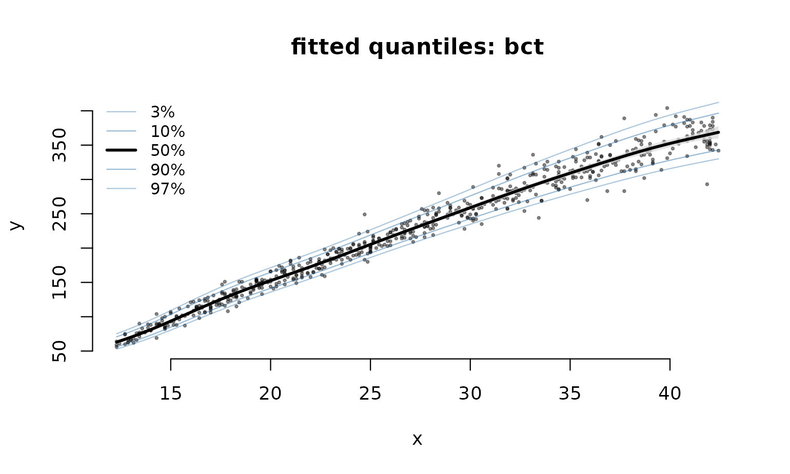
Four parameters: Box-Cox t on `abdom`

The LMS-style centile fit, and GAMLSS’s flagship. RTMBdist implements the same BCT density, to the digit:

c(RTMBdist = RTMBdist::dbct(60, 100, 0.1, 1, 5, log = TRUE),
  gamlss   = gamlss.dist::dBCT(60, 100, 0.1, 1, 5, log = TRUE))
#>  RTMBdist    gamlss 
#> -7.576373 -7.576373

t_gl <- tm(m3 <- gamlss(y ~ pb(x), sigma.fo = ~ pb(x), nu.fo = ~ 1,
                        tau.fo = ~ 1, family = BCT, data = abdom,
                        trace = FALSE))
t_rt <- tm(f3 <- gamRTMB(y ~ list(mu = ~ s(x), sigma = ~ s(x),
                                  nu = ~ 1, tau = ~ 1),
                         family = fam("bct"), data = abdom))

data.frame(
  fit     = c("gamlss", "gamRTMB"),
  seconds = round(c(t_gl, t_rt), 2),
  edf     = round(c(m3$df.fit, attr(edf(f3), "edf.total")), 2),
  AIC     = round(c(AIC(m3), AIC(f3)), 1)
)
#>       fit seconds   edf    AIC
#> 1  gamlss    0.38 11.76 4794.5
#> 2 gamRTMB    1.20 15.01 4803.5

Here the two part company a little. The fitted curves still agree —

p3 <- predict(f3, type = "response")
c(mu = cor(fitted(m3, "mu"), p3$mu), sigma = cor(fitted(m3, "sigma"), p3$sigma))
#>        mu     sigma 
#> 0.9999587 0.9990981

— but gamRTMB spends about three more effective degrees of freedom and pays for them in AIC. REML and GAMLSS’s criterion are choosing different amounts of smoothing on a 610-point dataset, and on this example GAMLSS chooses better. Worth knowing rather than glossing over.

plot(f3, type = "quantile", prob = c(0.03, 0.1, 0.5, 0.9, 0.97))

Fitted centile curves of abdominal circumference against gestational age, from the Box-Cox t model, over the data.

Where the two disagree: flat directions

The three examples so far are the ones GAMLSS was built for, and it handles them. The place the two approaches genuinely part company is a smooth on a parameter whose Fisher information collapses over part of its range.

GAMLSS fits by backfitting (the RS algorithm), which reweights the data by that information at every step and selects the smoothing parameter from those same weights. When the information goes to zero the weights collapse, the working response blows up, and the penalty cannot rein it back in because it was chosen from the degenerate weights. gamRTMB never forms a working weight: the smooth’s coefficients are integrated out by a Laplace approximation and the smoothing parameter comes from the resulting marginal likelihood, which stays finite in a flat direction instead of inverting it.

Both cases below are simulated, so we know the answer. The helper fits both packages on several data sets and records how often each converged and how far its fitted parameter lands from the truth.

compare <- function(nseed, sim, gfit, rfit, gpar, rpar, trans = identity) {
  one <- function(sx) {
    d <- sim(sx); conv <- TRUE
    g <- withCallingHandlers(tryCatch(gfit(d), error = function(e) NULL),
           warning = function(z) {
             if (grepl("converge", conditionMessage(z))) conv <<- FALSE
             invokeRestart("muffleWarning") })
    r <- tryCatch(suppressWarnings(rfit(d)), error = function(e) NULL)
    err <- function(v) if (is.null(v)) NA else
      sqrt(mean((trans(v) - trans(d$true))^2))
    c(!is.null(g) && conv && isTRUE(g$converged),
      !is.null(r) && isTRUE(r$convergence),
      err(if (is.null(g)) NULL else fitted(g, gpar)),
      err(if (is.null(r)) NULL else fitted(r)[[rpar]]))
  }
  z <- vapply(seq_len(nseed), one, numeric(4))
  data.frame(converged = paste0(rowSums(z[1:2, ]), "/", nseed),
             rmse = round(apply(z[3:4, ], 1, median), 2),
             row.names = c("gamlss", "gamRTMB"))
}

A smooth on the degrees of freedom of a t

The t density approaches a normal as its degrees of freedom grow, so the likelihood flattens out in that direction: the observed information for log(df) falls from 0.24 at df = 2 to 3e-4 at df = 100. Here the true df sweeps from 0.6 to 12 as a function of x, with location and scale held constant.

compare(10,
  function(sx) { set.seed(sx); x <- runif(200)
                 nu <- exp(1 + 1.5 * cos(2 * pi * x))
                 data.frame(x = x, true = nu, y = rTF(200, 0, 1, nu)) },
  function(d) gamlss(y ~ 1, sigma.fo = ~ 1, nu.fo = ~ pb(x),
                     family = TF, data = d, trace = FALSE),
  function(d) gamRTMB(y ~ list(mu = ~ 1, sigma = ~ 1, df = ~ s(x, k = 10)),
                      family = fam("t2"), data = d),
  "nu", "df", log)
#>         converged  rmse
#> gamlss       7/10 15.00
#> gamRTMB     10/10  0.71

The RMSE is on the log scale, so a value of 15 means the fitted degrees of freedom are out by a factor of exp(15). The failure is not confined to the runs GAMLSS flags: on five of the six runs it reports as converged, the fitted df still runs off past 1e11, and on one of them it reaches 3e221. Seed 8 is the clearest single case — GAMLSS spends 22.0 effective degrees of freedom to reach a log-likelihood of -436.3, where gamRTMB spends 3.5 and reaches -414.4. More flexibility, worse fit. Swapping the smoother does not help: pb(method = "GAIC") and a fixed-df cs() both diverge the same way, which is what points at the working weights rather than at the choice of penalty.

A skew normal with all three parameters smooth

compare(8,
  function(sx) { set.seed(sx); x <- runif(250); al <- 3 * sin(2 * pi * x)
                 data.frame(x = x, true = al,
                            y = rSN1(250, sin(2 * pi * x),
                                     exp(-0.5 + 0.6 * cos(2 * pi * x)), al)) },
  function(d) gamlss(y ~ pb(x), sigma.fo = ~ pb(x), nu.fo = ~ pb(x),
                     family = SN1, data = d, trace = FALSE),
  function(d) gamRTMB(y ~ list(mean = ~ s(x, k = 10), sd = ~ s(x, k = 10),
                               alpha = ~ s(x, k = 10)),
                      family = fam("skewnorm2"), data = d),
  "nu", "alpha")
#>         converged rmse
#> gamlss        2/8 2.25
#> gamRTMB       6/8 1.95

The slant is the flat direction here: the score for it vanishes identically at zero skewness, so the surface has a plateau exactly where a fit is likely to start. GAMLSS rarely gets off it. Its fitted slant stays inside 0.4 in absolute value against a truth ranging over 3, which is why its RMSE of 2.25 is no better than the 2.12 you would score by giving up and fitting no skewness at all — and it spends 15 to 18 effective degrees of freedom doing it. gamRTMB recovers roughly the right amplitude, though it is not comfortable here either: it fails to converge on some runs and overshoots the slant on others. This is a hard likelihood for anything.

Speed

One run each on one machine, so read these as orders of magnitude rather than benchmarks. Dutch boys’ BMI against age, normal location-scale, at three sample sizes:

data(dbbmi)
sizes <- c(500, 2000, nrow(dbbmi))
res <- t(vapply(sizes, function(n) {
  d <- if (n == nrow(dbbmi)) dbbmi else
    { set.seed(1); dbbmi[sort(sample(nrow(dbbmi), n)), ] }
  c(gamlss  = tm(gamlss(bmi ~ pb(age), sigma.fo = ~ pb(age), data = d,
                        trace = FALSE)),
    gamRTMB = tm(gamRTMB(bmi ~ list(mean = ~ s(age), sd = ~ s(age)), data = d)))
}, c(gamlss = 0, gamRTMB = 0)))
data.frame(n = sizes, round(res, 2))
#>      n gamlss gamRTMB
#> 1  500   0.40    0.35
#> 2 2000   0.37    0.95
#> 3 7294   3.83    2.37

Neither dominates. Both stay within about a factor of two of each other across this range, and which one is ahead is not even monotone in n — which is itself the finding: the differences are small enough that a single run cannot separate them, and no scaling story should be read into three points this close. Speed is not a reason to pick either package here.

What actually differs

Where gamRTMB gives you something else:

Parameter names and count. GAMLSS is capped at four parameters called mu, sigma, nu, tau; gamRTMB has no cap and uses each density’s own names — hence mean/sd for a Gaussian and xi/omega/alpha for a skew normal. The rent example shows why that matters: GA’s sigma is a coefficient of variation, and a generic name hides it.
mgcv’s smooths. s(), t2(), by= factors, bs="fs", bs="re", shrinkage bases, and id= to share a smoothing parameter between terms and between distributional parameters.
Exact derivatives, by automatic differentiation rather than analytic or numerical ones supplied per family.
Flat directions, as above: no working weights to collapse, so a smooth on a weakly identified parameter degrades rather than diverges.

Where GAMLSS is ahead today: term selection (stepGAIC), distribution search (fitDist, chooseDist), censoring and truncation of arbitrary families (gamlss.cens, gamlss.tr), finite mixtures, and twenty years of use. If you need those, use GAMLSS.

Normal location-scale: abdom

Gamma: rent

Four parameters: Box-Cox t on abdom