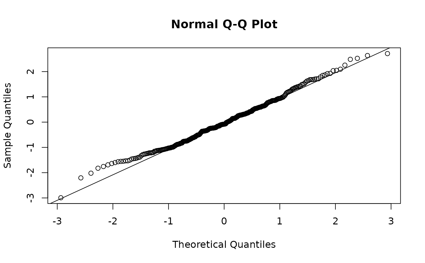
Randomised quantile (pseudo) residuals — residuals.gamRTMB • gamRTMB

Residuals by the probability integral transform: if the fitted distribution is right, $u_i = F(y_i; \hat\theta_i)$ is uniform and $r_i = \Phi^{-1}(u_i)$ is standard normal, so a QQ plot of r checks the whole distributional assumption rather than just the mean.

Usage

# S3 method for class 'gamRTMB'
residuals(object, type = c("quantile", "uniform"), randomise = TRUE, ...)

Arguments

object: A gamRTMB fit.
type: "quantile" for normal-scale residuals (the default), or "uniform" for the PIT values themselves.
randomise: Randomise within the step for a discrete or mixed response. Ignored for a continuous one.
...: Ignored.

Value

A numeric vector, or with randomise = FALSE and a non-continuous response a data frame of lower, upper and mid. Values are clamped away from 0 and 1 so that extreme observations stay finite and visible.

Discrete and mixed responses

Where the response has atoms, $F$ is a step function and $u$ cannot be uniform, so the residual is randomised within the step (Dunn & Smyth 1996): $$u_i = F(y_i^-) + v_i (F(y_i) - F(y_i^-)), \quad v_i \sim U(0,1).$$ The left limit $F(y^-)$ comes from the family's declared support, since it cannot be obtained reliably any other way:

continuous: $F(y^-) = F(y)$ and no randomisation happens.
lattice: $F(y^-) = F(y-1)$, evaluated at integer arguments only, and taken as 0 at $y = 0$ rather than evaluating the CDF below its support.
mixed: $F(y^-) = F(y) - p(y)$ at an atom, where the density returns the atom's mass, and $F(y)$ elsewhere.

Nudging the argument instead ($F(y-\delta)$) is not safe: CDF implementations disagree about whether they floor a non-integer argument, and some reject one outright.

Randomisation

With randomise = TRUE (the default, and what you want for a QQ plot) the residuals are not a deterministic function of the fit; set a seed for reproducibility, or inspect several draws. With randomise = FALSE a discrete or mixed response returns the bounding interval per observation instead of a point.

Prior weights are ignored: a residual belongs to a row of the data, not to the replicate count a weight stands for.

References

Dunn, P. K. and Smyth, G. K. (1996) Randomized quantile residuals. Journal of Computational and Graphical Statistics 5, 236–244.

Examples

set.seed(1)
d <- data.frame(x = runif(300))
d$y <- rpois(300, exp(1 + sin(2 * pi * d$x)))
fit <- gamRTMB(y ~ list(lambda = ~ s(x, k = 8)), family = fam("pois"),
               data = d)
r <- residuals(fit)
qqnorm(r); qqline(r)