Build a LaMaModel from an optimised RTMB object

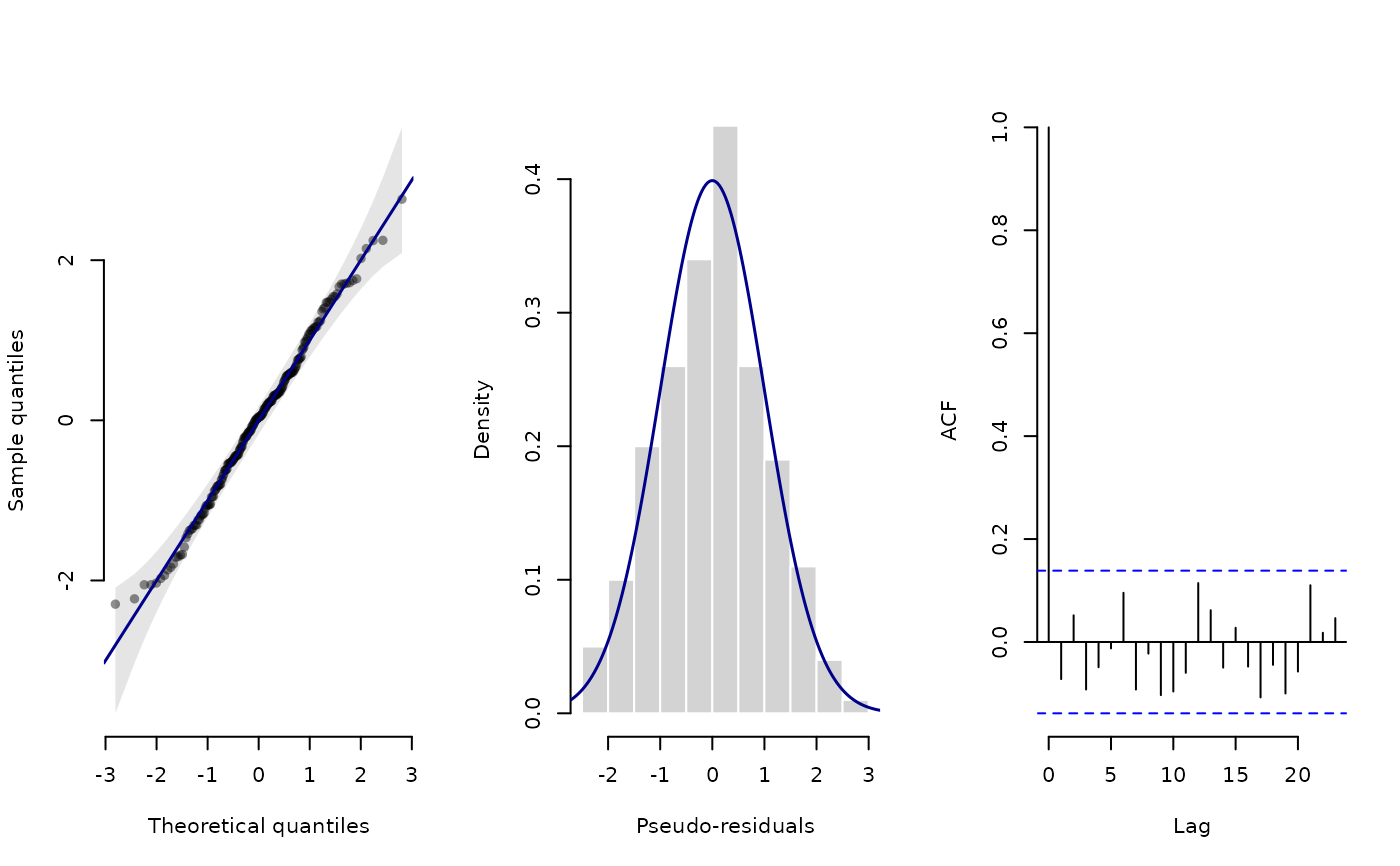
Having fitted a latent Markov model using automatic differentiation via RTMB, this function calls RTMB's obj$report() and does some additional processing. This then yields estimated parameters on their natural scale, allows for convenient calculation of AIC and BIC, state-decoding, and residual calculation. print() gives a short overview of the model, summary() the estimates. report() is the deprecated old name of lama().

Usage

lama(obj)

report(obj)

Arguments

obj

Optimised RTMB object

Value

A model object of class "LaMaModel" containing a list with the reported quantities from the RTMB object, along estimated parameters (par), the log-likelihood (llk), number of parameters (df) and observations (nobs), and the maximum gradient component (mgc) at the estimate. It also contains obj itself (not a copy), so that functions like MCreport or scores can be called on the model object.

Details

The number of observations (used by BIC) is the number of rows of the reported allprobs that are not all 1, i.e. missing observations are not counted. This assumes that forward is called only once in the likelihood function.

Examples

data <- trex[1:200,]

# initial parameters and observations
par <- list(
  log_mu = log(c(0.3, 1)),      # initial means for step length (log-transformed)
  log_sigma = log(c(0.2, 0.7)), # initial sds for step length (log-transformed)
  eta = rep(-2, 2)              # initial t.p.m. parameters (on logit scale)
)    
dat <- list(
  step = data$step,             # hourly step lengths
  nStates = 2                   # number of hidden states
)

# likelihood function
nll <- function(par) {
  getAll(par, dat)
  Gamma <- tpm(eta)
  delta <- stationary(Gamma)
  mu <- exp(log_mu); REPORT(mu)
  sigma <- exp(log_sigma); REPORT(sigma)
  allprobs <- matrix(1, length(step), nStates)
  ind <- which(!is.na(step))
  for(j in 1:nStates) {
    allprobs[ind,j] <- dgamma2(step[ind], mu[j], sigma[j]) 
  } 
  -forward(delta, Gamma, allprobs)
}

# automatic differentiation and optimisation
obj <- MakeADFun(nll, par, silent = TRUE)
opt <- nlminb(obj$par, obj$fn, obj$gr)

### reporting ###
mod <- lama(obj)
mod          # short overview
#> Latent Markov model with 2 states (discrete time, homogeneous)
#> 200 observations, 6 parameters
#> Log-likelihood: -210.27   AIC: 432.53   BIC: 452.32
#> Reported: mu, sigma, delta, Gamma, allprobs
summary(mod) # estimated state process and reported quantities
#> Latent Markov model with 2 states (discrete time, homogeneous)
#> 200 observations, 6 parameters
#> 
#> Transition probability matrix:
#>        S1     S2
#> S1 0.8085 0.1915
#> S2 0.2256 0.7744
#> 
#> Stationary distribution:
#>     S1     S2 
#> 0.5409 0.4591 
#> 
#> Mean dwell times:
#>    S1    S2 
#> 5.223 4.433 
#> 
#> Reported quantities:
#>           S1    S2
#> mu    0.3136 2.568
#> sigma 0.2034 1.514
#> 
#> Log-likelihood: -210.27   AIC: 432.53   BIC: 452.32
#> Maximum gradient component: 0.000444

# estimated parameters
mod$par
#> $log_mu
#> [1] -1.1595375  0.9430611
#> 
#> $log_sigma
#> [1] -1.5925839  0.4146816
#> 
#> $eta
#> [1] -1.233553 -1.440485
#> 
#> attr(,"check.passed")
#> [1] TRUE

# estimated quantities on natural scale
mod$mu
#> [1] 0.3136312 2.5678297
mod$sigma
#> [1] 0.2033994 1.5138886
mod$Gamma
#>           S1        S2
#> S1 0.8085298 0.1914702
#> S2 0.2255601 0.7744399

# information criteria
AIC(mod)
#> [1] 432.5328
BIC(mod)
#> [1] 452.3227

# state decoding
states <- viterbi(mod = mod)   # global decoding
probs <- stateprobs(mod = mod) # local decoding

# residual calculation
pres <- pseudo_res(data$step, # observation sequence
                   "gamma2",  # distribution family
                   list(mean = mod$mu, sd = mod$sigma), # parameters for that family
                   mod = mod) # model object

# or from the model object alone, and plotted
plot(mod)