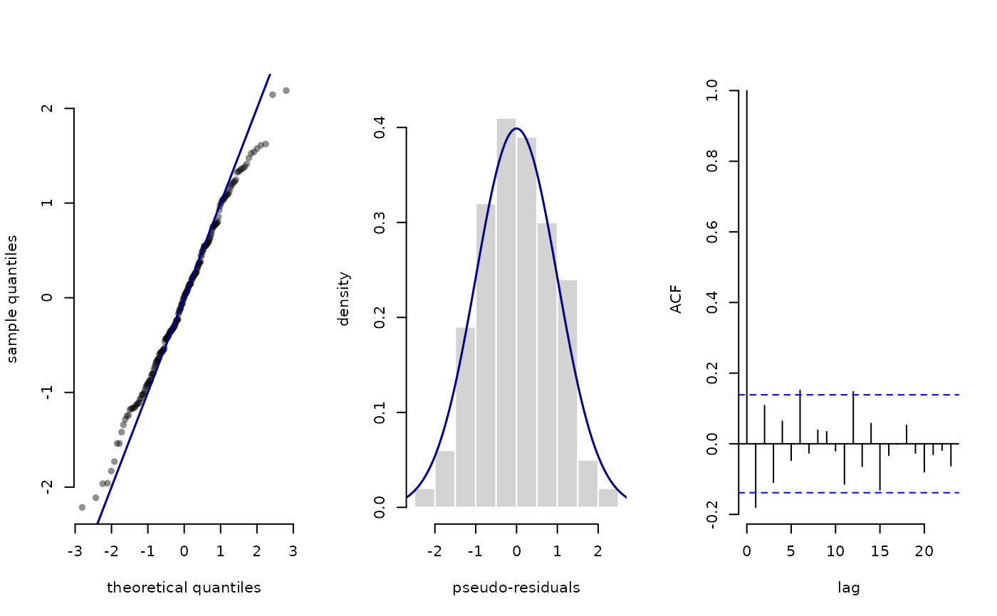
Calculate pseudo-residuals

For HMMs, pseudo-residuals are used to assess the overall goodness-of-fit of the model. These are based on the cumulative distribution function (CDF) $$F_{X_t}(x_t) = F(x_t \mid x_1, \dots, x_{t-1})$$ and can be used to quantify whether an observation is extreme relative to its model-implied distribution.

This function calculates such residuals via the probability integral transform, based on the local state probabilities obtained by stateprobs or stateprobs_g and the respective parametric family.

Usage

pseudo_res(
  obs,
  dist,
  par,
  stateprobs = NULL,
  mod = NULL,
  normal = TRUE,
  discrete = NULL,
  randomise = TRUE
)

Arguments

obs

vector of continuous-valued observations (of length nObs)

dist

character string specifying which parametric CDF to use (e.g., "norm" for normal or "pois" for Poisson) or CDF function to evaluate directly. If a discrete CDF function is passed, the discrete argument needs to be set to TRUE because this cannot determined automatically.

par

named parameter list for the parametric CDF

Names need to correspond to the parameter names in the specified distribution (e.g. list(mean = c(1,2), sd = c(1,1)) for a normal distribution and 2 states). This argument is as flexible as the parametric distribution allows. For example you can have a matrix of parameters with one row for each observation and one column for each state.

stateprobs

matrix of local state probabilities for each observation (of dimension c(nObs, nStates)) as computed by stateprobs, stateprobs_g or stateprobs_p

mod

optional model object containing required quantities

When using automatic differentiation either with RTMB::MakeADFun or qreml and include forward, forward_g or forward_p in your likelihood function, the objects needed for state decoding are automatically reported after model fitting. Hence, you can pass the model object obtained from running report() or from qreml directly to this function and avoid calculating local state proabilities manually. In this case, a call should look like pseudo_res(obs, "norm", par, mod = mod).

normal

logical, if TRUE, returns Gaussian pseudo residuals

These will be approximately standard normally distributed if the model is correct.

discrete

logical, if TRUE, computes discrete pseudo residuals (which slightly differ in their definition)

By default, will be determined using dist argument, but only works for standard discrete distributions. When used with a special discrete distribution, set to TRUE manually.

randomise

for discrete pseudo residuals only. Logical, if TRUE, return randomised pseudo residuals. Recommended for discrete observations.

Value

vector of pseudo residuals of class LaMaResiduals or list containing lower, upper, and mean if discrete residuals are not randomised.

Details

Pseudo-residuals are based on the probability integral transform. If the cumulative distribution function (CDF) $F$ of a random variable $X$ is known, then $F(X)$ is uniformly distributed on $[0,1]$. Applying the standard normal quantile function $\Phi^{-1}$ then gives a residual that is approximately standard normal under the model.

For discrete-valued observations, the CDF is a step function, so the residual is not uniquely defined. One can compute a "lower" and "upper" pseudo-residual corresponding to $F(X-1)$ and $F(X)$, respectively. If randomise = TRUE, a value is drawn uniformly between the lower and upper bounds. In this case, the resulting pseudo-residuals are again approximately standard normal after applying the standard normal quantile function.

Examples

## continuous-valued observations
obs = rnorm(100)
stateprobs = matrix(0.5, nrow = 100, ncol = 2)
par = list(mean = c(1,2), sd = c(1,1))
pres = pseudo_res(obs, "norm", par, stateprobs)

## discrete-valued observations
obs = rpois(100, lambda = 1)
par = list(lambda = c(1,2))
pres = pseudo_res(obs, "pois", par, stateprobs)
#> Calculating discrete pseudo-residuals
#> Randomised between lower and upper

## custom CDF function
obs = rnbinom(100, size = 1, prob = 0.5)
par = list(size = c(0.5, 2), prob = c(0.4, 0.6))
pres = pseudo_res(obs, pnbinom, par, stateprobs, 
                  discrete = TRUE)
#> Calculating discrete pseudo-residuals
#> Randomised between lower and upper
# if discrete CDF function is passed, 'discrete' needs to be set to TRUE

## no CDF function available, only density (artificial example)
obs = rnorm(100)
par = list(mean = c(1,2), sd = c(1,1))
# construct CDF using numerical integration
cdf = function(x, mean, sd) integrate(dnorm, -Inf, x, mean = mean, sd = sd)$value
pres = pseudo_res(obs, cdf, par, stateprobs)
#> Assuming 'dist' evaluates a continuous CDF. Set 'discrete = TRUE' if not.


### Full model fit example ###
step = trex$step[1:200]

nll = function(par){
  getAll(par)
  Gamma = tpm(logitGamma)
  delta = stationary(Gamma)
  mu = exp(logMu); REPORT(mu)
  sigma = exp(logSigma); REPORT(sigma)
  allprobs = matrix(1, length(step), 2)
  ind = which(!is.na(step))
  for(j in 1:2) allprobs[ind,j] = dgamma2(step[ind], mu[j], sigma[j])
  -forward(delta, Gamma, allprobs)
}

par = list(logitGamma = c(-2,-2), 
           logMu = log(c(0.3, 2.5)), 
           logSigma = log(c(0.3, 0.5)))
           
obj = MakeADFun(nll, par, silent = TRUE)
opt = nlminb(obj$par, obj$fn, obj$gr)

mod = obj$report()

pres = pseudo_res(step,      # observation sequence
                  "gamma2",  # parametric family that was used
                  list(mean = mod$mu, sd = mod$sigma), # parameters for that family
                  mod = mod) # model object

plot(pres)

Usage

Arguments

Value

Details

See also

Examples