Plot pseudo-residuals
plot.LaMaResiduals.RdPlot pseudo-residuals computed by pseudo_res.
Arguments
- x
pseudo-residuals as returned by
pseudo_res- col
character, color for the QQ-line (and density curve if
histogram = TRUE)- lwd
numeric, line width for the QQ-line (and density curve if
histogram = TRUE)- main
optional character vector of main titles for the plots of length 2 (or 3 if
histogram = TRUE)- breaks
breaksargument passed to hist- axis.lab
labels used for the x and y axis of each plot (named list)
- ...
currently ignored. For method consistency
Examples
## pseudo-residuals for the trex data
step = trex$step[1:1000]
angle = trex$angle[1:1000]
nll = function(par){
getAll(par)
Gamma = tpm(logitGamma)
delta = stationary(Gamma)
mu = exp(logMu); REPORT(mu)
sigma = exp(logSigma); REPORT(sigma)
kappa = exp(logKappa); REPORT(kappa)
allprobs = matrix(1, length(step), 2)
ind = which(!is.na(step) & !is.na(angle))
for(j in 1:2) {
allprobs[ind,j] = dgamma2(step[ind], mu[j], sigma[j]) *
dvm(angle[ind], 0, kappa[j])
}
-forward(delta, Gamma, allprobs)
}
par = list(logitGamma = c(-2,-2),
logMu = log(c(0.3, 2.5)),
logSigma = log(c(0.3, 0.5)),
logKappa = log(c(0.2, 1)))
obj = MakeADFun(nll, par, silent = TRUE)
opt = nlminb(obj$par, obj$fn, obj$gr)
mod = report(obj)
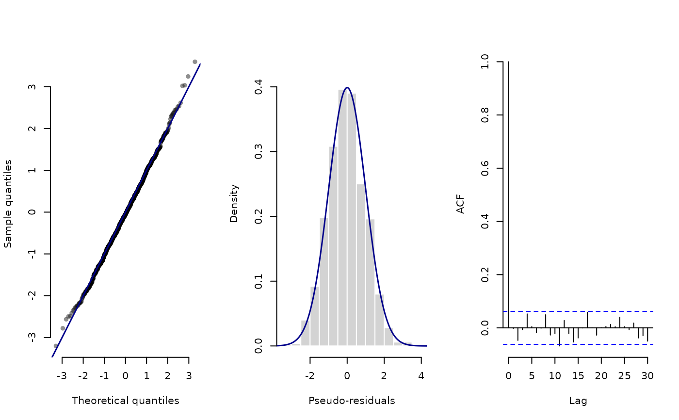
pres_step = pseudo_res(step, # observations
"gamma2", # family that is used
list(mean = mod$mu, sd = mod$sigma), # the family's parameters
mod = mod) # model object
pres_angle = pseudo_res(angle,
"vm",
list(mu = 0, kappa = mod$kappa),
mod = mod)
# separate plots
plot(pres_step)
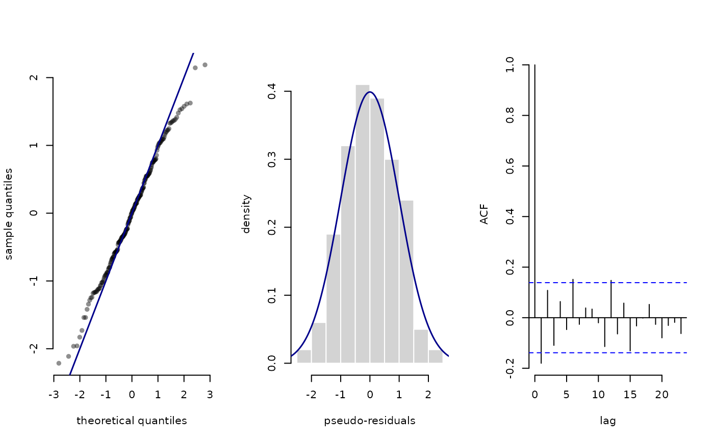 plot(pres_angle)
 # together
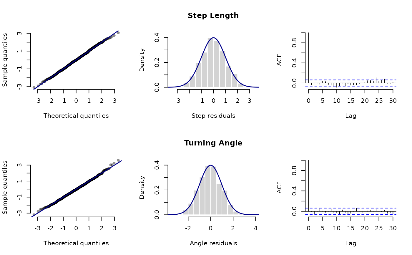
par(mfrow = c(2,3))
plot(pres_step, main = c("", "Step Length", ""),
axis.lab = list(hist = c("Step residuals", "Density")))
plot(pres_angle, main = c("", "Turning Angle", ""),
axis.lab = list(hist = c("Angle residuals", "Density")))
# together
par(mfrow = c(2,3))
plot(pres_step, main = c("", "Step Length", ""),
axis.lab = list(hist = c("Step residuals", "Density")))
plot(pres_angle, main = c("", "Turning Angle", ""),
axis.lab = list(hist = c("Angle residuals", "Density")))