2 Finer control

Before diving into this vignette, we recommend reading the vignette Introduction to LaMa.

In the introduction, we used a few shortcuts: statedens() built the matrix of state-dependent densities, forward("stationary", ...) computed the initial distribution, and lama() gave us a model object for decoding, residuals and plots. Each of them is code you can also write yourself – with automatic differentiation just as without – which gives arbitrarily fine control. You need this as soon as a model does not fit the shortcuts, e.g. for a custom initial distribution, densities transformed by hand, or other model classes like continuous-time HMMs, state space models or hidden semi-Markov models.

In this vignette, we first explain how the HMM likelihood is computed and fit a simple HMM without automatic differentiation to see all building blocks at work. We then write the likelihood of the trex model from the introduction by hand, using RTMB as before.

library(LaMa)
#> Loading required package: RTMB

The HMM likelihood

Computing the HMM likelihood for observations x_1, \dots, x_T is non-trivial, as we do not observe the underlying states and need to sum out all possible state sequences. Exploiting the Markov property, the so-called forward algorithm does this recursively as a matrix product:

L(\boldsymbol{\theta}) = \boldsymbol{\delta}^{(1)} \boldsymbol{P}(x_1) \boldsymbol{\Gamma} \boldsymbol{P}(x_2) \boldsymbol{\Gamma} \dots \boldsymbol{\Gamma} \boldsymbol{P}(x_T) \boldsymbol{1}^\top, where \boldsymbol{\delta}^{(1)} and \boldsymbol{\Gamma} are the initial distribution and the transition probability matrix, \boldsymbol{P}(x_t) is a diagonal matrix with the state-dependent densities (or probability mass functions) f_j(x_t) = f(x_t \mid S_t = j) on its diagonal, \boldsymbol{1} is a row vector of ones and \boldsymbol{\theta} contains all model parameters. In practice, forward() does not compute this likelihood directly, but its logarithm via a scaling strategy (Zucchini et al. 2016).

Many parameters are constrained, e.g. standard deviations are positive and the rows of the transition probability matrix sum to one. Instead of constrained optimisation, we maximise the likelihood w.r.t. unconstrained parameters (par in the code), which are transformed by link functions: e.g. the log link for positive parameters and the multinomial logistic link (softmax) for the transition probability matrix, implemented in tpm().

For efficiency, the state-dependent densities are evaluated vectorised before running the forward algorithm. This gives a matrix with one row per observation and one column per state, which, throughout the package, we call the allprobs matrix.

Fitting an HMM without automatic differentiation

forward() and the other building blocks also work without automatic differentiation. They are then still worth using: without AD, forward() runs in C++, as does tpm() for many time-varying transition probability matrices, which is much faster than writing the forward algorithm yourself in R. To see all parts in action, we simulate data from a 2-state HMM with Gaussian state-dependent distributions and fit it with nlm().

Generating data from a 2-state HMM

# parameters
mu = c(0, 6)    # state-dependent means
sigma = c(2, 4) # state-dependent standard deviations
Gamma = matrix(c(0.95, 0.05, # transition probability matrix
                 0.15, 0.85),
               nrow = 2, byrow = TRUE)
delta = stationary(Gamma) # stationary distribution

# simulation
n = 1000
set.seed(123)
s = rep(NA, n)
s[1] = sample(1:2, 1, prob = delta) # sampling first state from delta
for(t in 2:n){
  # drawing the next state conditional on the last one
  s[t] = sample(1:2, 1, prob = Gamma[s[t-1],])
}
# drawing the observation conditional on the states
x = rnorm(n, mu[s], sigma[s]) # independent given the state sequence

color = LaMaColors(2)
plot(x[1:200], bty = "n", pch = 20, ylab = "x",
     col = color[s[1:200]])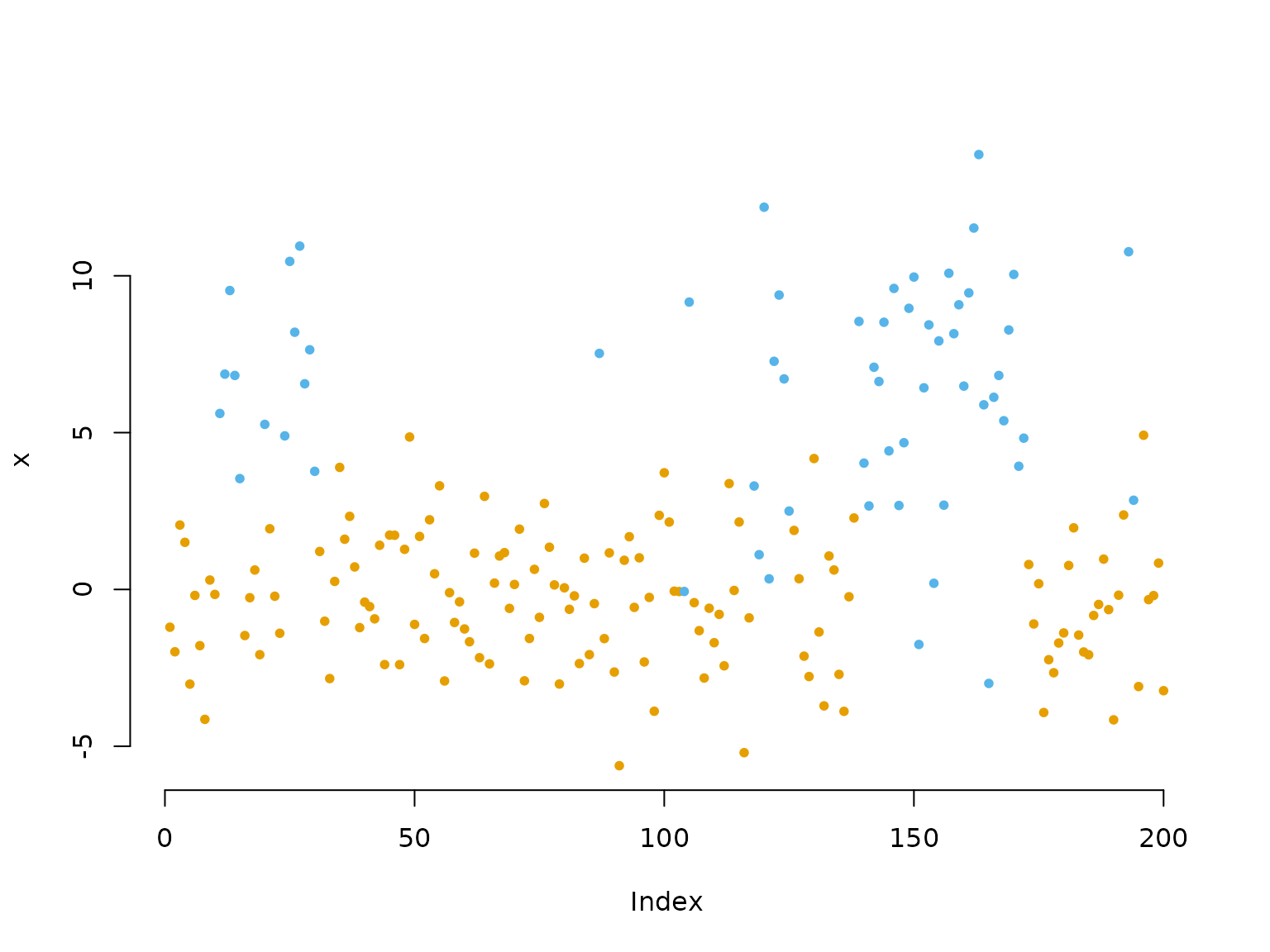

Inference by direct numerical maximum likelihood estimation

Within the negative log-likelihood function we

build the transition probability matrix using the tpm() function,
compute the stationary distribution of the Markov chain using stationary(),
build the allprobs matrix, and
calculate the log-likelihood using forward(), returning -1 times it for minimisation.

nll = function(par, x){
  # 1) Transition probability matrix
  Gamma = tpm(par[1:2]) # multinomial logistic link (softmax)
  # 2) Stationary distribution for this matrix
  delta = stationary(Gamma) # will be used as initial
  # Parameter transformations for unconstrained optimisation
  mu = par[3:4] # no transformation needed
  sigma = exp(par[5:6]) # strictly positive
  # 3) Calculating state-dependent densities outside the forward algorithm
  allprobs = matrix(1, length(x), 2)
  for(j in 1:2) allprobs[,j] = dnorm(x, mu[j], sigma[j])
  # 4) Run the forward algorithm
  -forward(delta, Gamma, allprobs)
}

The shortcut statedens(x, dnorm, mu, sigma) would give the same matrix as the loop in step 3, and forward("stationary", Gamma, allprobs) would replace step 2.

We fit the model with nlm(), starting from initial values on the unconstrained scale. As tpm() uses the softmax link, an off-diagonal probability p corresponds to the starting value qlogis(p); here we start near 0.05. In practice, it is advisable to try several sets of initial values to find the global maximum.

par = c(logitGamma = qlogis(c(0.05, 0.05)),
        mu = c(1,4),
        logsigma = c(log(1),log(3)))
# initial transformed parameters: not chosen too well
system.time(
  opt <- nlm(nll, par, x = x)
)
#>    user  system elapsed 
#>   0.132   0.006   0.138

This is fast because forward() runs in C++. With the forward algorithm written in R, the same fit takes roughly three times as long.

With AD, we can use the same likelihood function, only wrapped into a function of a parameter list:

system.time({
  obj = MakeADFun(function(p) nll(p$par, x), list(par = par), silent = TRUE)
  opt_ad <- nlminb(obj$par, obj$fn, obj$gr)
})
#>    user  system elapsed 
#>   0.143   0.000   0.143

For such a small and simple model, it hardly matters whether we use AD. For larger models, however, it matters a lot: without AD, the gradient is approximated by finite differences, which costs one additional likelihood evaluation per parameter and is less accurate. For example, a 3-state model for the trex step lengths and turning angles (15 parameters) takes about 8 seconds to fit without and about 1 second with AD. The exact gradient also makes the optimisation numerically more stable.

Visualising results

Without RTMB, there is no model object, so we need to back-transform the estimated parameters ourselves, as in the likelihood:

estimate = opt$estimate
# transform parameters to natural scale
Gamma = tpm(estimate[1:2])
delta = stationary(Gamma) # stationary HMM
mu = estimate[3:4]
sigma = exp(estimate[5:6])

hist(x, prob = TRUE, bor = "white", breaks = 40, main = "")
curve(delta[1]*dnorm(x, mu[1], sigma[1]), add = TRUE, lwd = 2, col = color[1], n=500)
curve(delta[2]*dnorm(x, mu[2], sigma[2]), add = TRUE, lwd = 2, col = color[2], n=500)
curve(delta[1]*dnorm(x, mu[1], sigma[1])+delta[2]*dnorm(x, mu[2], sigma[2]),
      add = TRUE, lwd = 2, lty = "dashed", n=500)
legend("topright", col = c(color, "black"), lwd = 2, bty = "n",
       lty = c(1,1,2), legend = c("state 1", "state 2", "marginal"))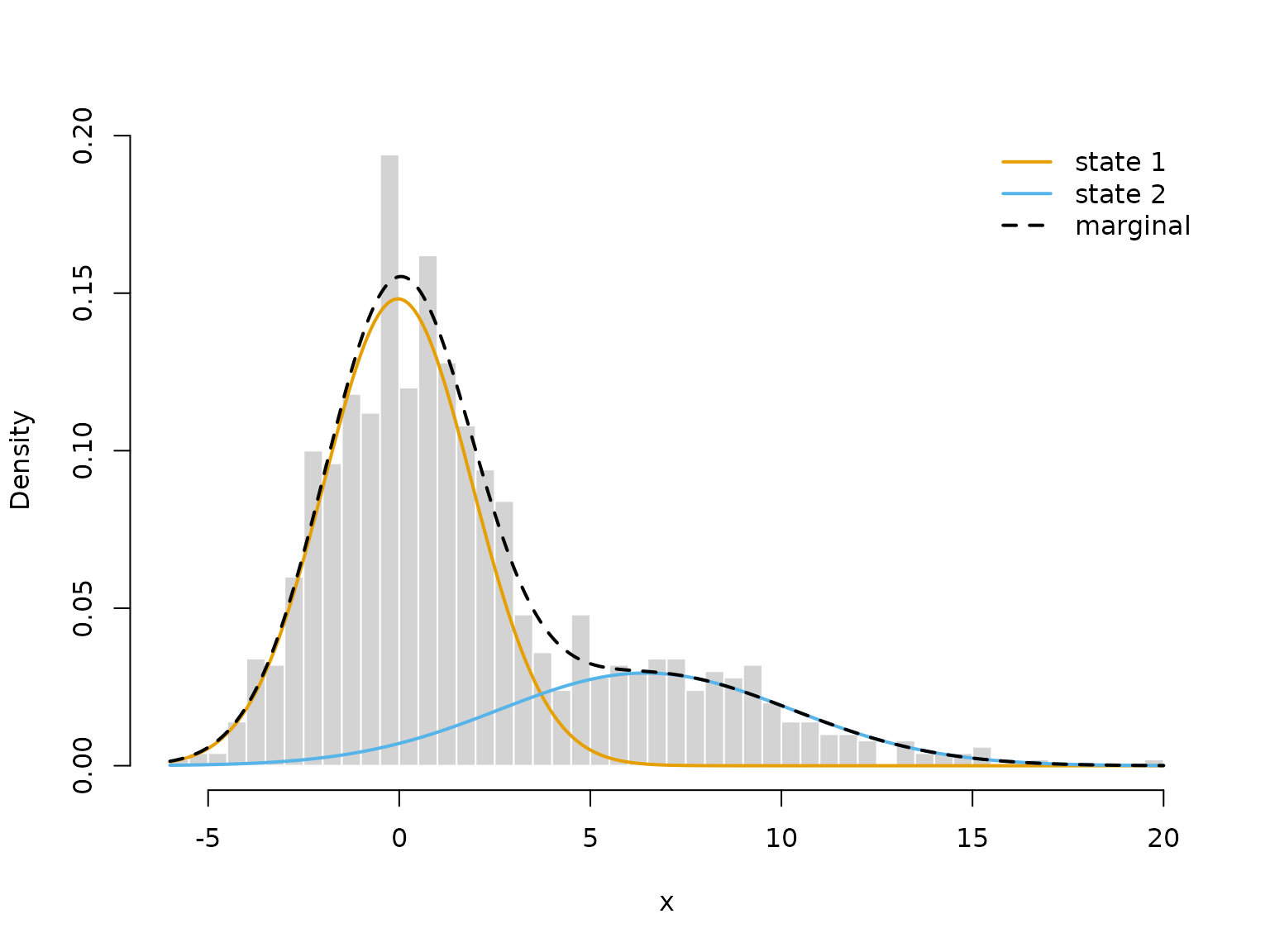

To decode the most probable state sequence with viterbi(), we first compute the allprobs matrix:

allprobs = matrix(1, length(x), 2)
for(j in 1:2) allprobs[,j] = dnorm(x, mu[j], sigma[j])

states = viterbi(delta, Gamma, allprobs)

plot(x, pch = 20, bty = "n", col = color[states])
legend("topright", pch = 20, legend = c("state 1", "state 2"),
       col = color, box.lwd = 0)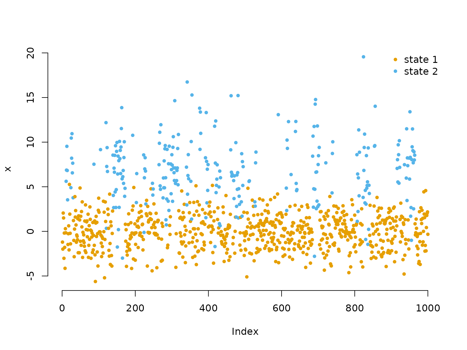

For pseudo-residuals, pseudo_res() needs the observations, the parametric family, the estimated parameters and the local state probabilities:

probs = stateprobs(delta, Gamma, allprobs) # local state probabilities

pres = pseudo_res(x, # observations
                  "norm", # parametric distribution to use
                  list(mean = mu, sd = sigma), # parameters for that distribution
                  probs) # local state probabilities

# use the plotting method for LaMaResiduals
plot(pres)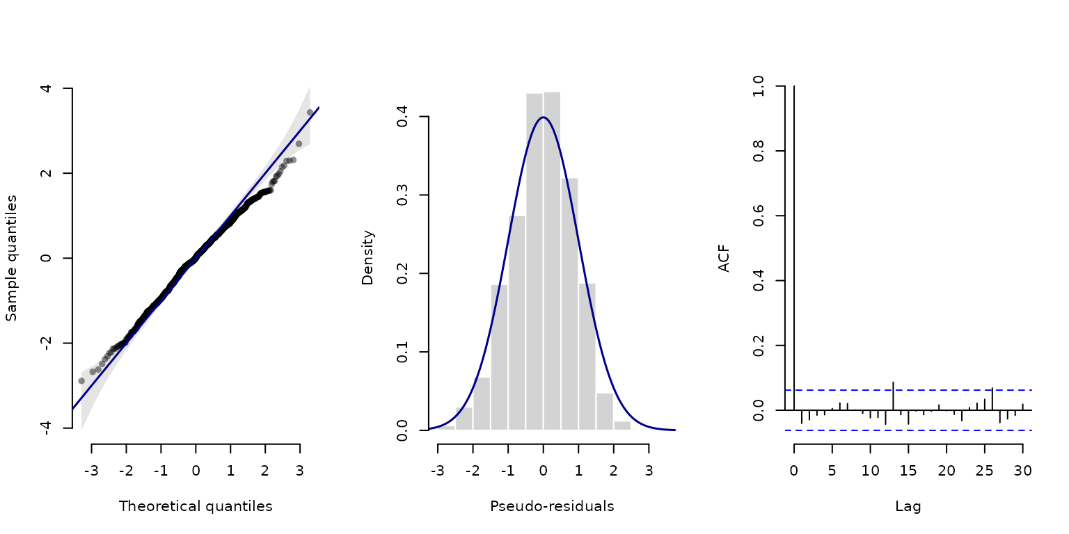

In this case, our model looks really good – which it should because it is correctly specified.

Writing everything yourself with RTMB

Writing the likelihood explicitly works just the same with automatic differentiation. We return to the trex model from the introduction:

par = list(
  log_mu = log(c(0.3, 1)),      # initial means for step length (log-transformed)
  log_sigma = log(c(0.2, 0.7)), # initial sds for step length (log-transformed)
  eta = rep(-2, 2)              # initial t.p.m. parameters (on logit scale)
  )

dat = list(
  step = trex$step,   # hourly step lengths
  N = 2
  )

This time, we compute the stationary distribution with stationary() and build allprobs with a loop over states. Rows of missing observations stay 1, such that they do not contribute to the likelihood – exactly what statedens() does.

nll2 = function(par) {
  getAll(par, dat) # makes everything contained available without $
  Gamma = tpm(eta) # computes transition probability matrix from unconstrained eta
  delta = stationary(Gamma) # computes stationary distribution
  # Parameter transformations for strictly positive parameters
  mu = exp(log_mu)
  sigma = exp(log_sigma)
  # Reporting statements for later use
  REPORT(mu); ADREPORT(mu)
  REPORT(sigma); ADREPORT(sigma)
  # Calculating all state-dependent densities
  allprobs = matrix(1, nrow = length(step), ncol = N)
  ind = which(!is.na(step)) # only for non-NA obs.
  for(j in 1:N){
    allprobs[ind,j] = dgamma2(step[ind], mu[j], sigma[j])
  }
  -forward(delta, Gamma, allprobs) # simple forward algorithm
}

obj2 = MakeADFun(nll2, par, silent = TRUE)
opt2 = nlminb(obj2$par, obj2$fn, obj2$gr)
mod2 = lama(obj2)

This gives the same fit as the short version in the introduction:

-opt2$objective
#> [1] -10847.12
mod2$Gamma
#>           S1        S2
#> S1 0.8269542 0.1730458
#> S2 0.1608473 0.8391527

Writing the likelihood explicitly gives full control over each part. Throughout the vignettes, you will see examples of this, e.g.

a custom initial distribution, like an estimated one for inhomogeneous models (see Extensions),
the periodically stationary distribution computed by stationary_p() instead of forward("stationary", ..., tod = tod), to report it for all times of day (see Extensions),
state-dependent densities transformed by hand, e.g. for zero-inflation or smooth densities (see Penalised splines), or
transition probability matrices computed in a different way, e.g. for continuous-time HMMs or hidden semi-Markov models.

Downstream functions

With automatic differentiation, forward() always reports delta, Gamma and allprobs, no matter how they were computed. The viterbi() and stateprobs() functions either take these as arguments or, more conveniently, the whole reported mod object as an input:

states = viterbi(mod2$delta, mod2$Gamma, mod2$allprobs)
all.equal(states, viterbi(mod2))
#> [1] TRUE

For this to work, forward() should only be called once in the likelihood function, with the trackID argument for several tracks (see the vignette on Longitudinal data).

pseudo_res(mod) evaluates the likelihood function again with the densities replaced by their CDFs, which also works with an allprobs matrix built by hand. Alternatively, we can specify the observations, the parametric family and the estimated parameters manually:

pres_step = pseudo_res(obs = trex$step, # observation sequence
                       dist = "gamma2", # which parametric CDF to use
                       par = list(mean = mod2$mu, sd = mod2$sigma), # estimated pars for that CDF
                       mod = mod2) # model object
all.equal(pres_step, pseudo_res(mod2))
#> [1] TRUE

This is needed when the densities are transformed by hand inside the likelihood, e.g. for zero-inflation, where swapping in CDFs is not valid. plot(pres_step) then gives the same plots as plot(mod2).

Similarly, plot(mod, type = "statedens") needs the information recorded by statedens(). With a hand-built allprobs matrix, we plot the estimated state-dependent distributions ourselves:

delta = mod2$delta
mu = mod2$mu
sigma = mod2$sigma

hist(trex$step, prob = TRUE, breaks = 40,
     bor = "white", main = "", xlab = "step length")
for(j in 1:2) curve(delta[j] * dgamma2(x, mu[j], sigma[j]),
                    lwd = 2, add = TRUE, col = color[j])
curve(delta[1]*dgamma2(x, mu[1], sigma[1]) + delta[2]*dgamma2(x, mu[2], sigma[2]),
      lwd = 2, lty = 2, add = TRUE)
legend("top", lwd = 2, lty = c(1, 1, 2), col = c(color, "black"), bty = "n",
       legend = c("state 1", "state 2", "marginal"))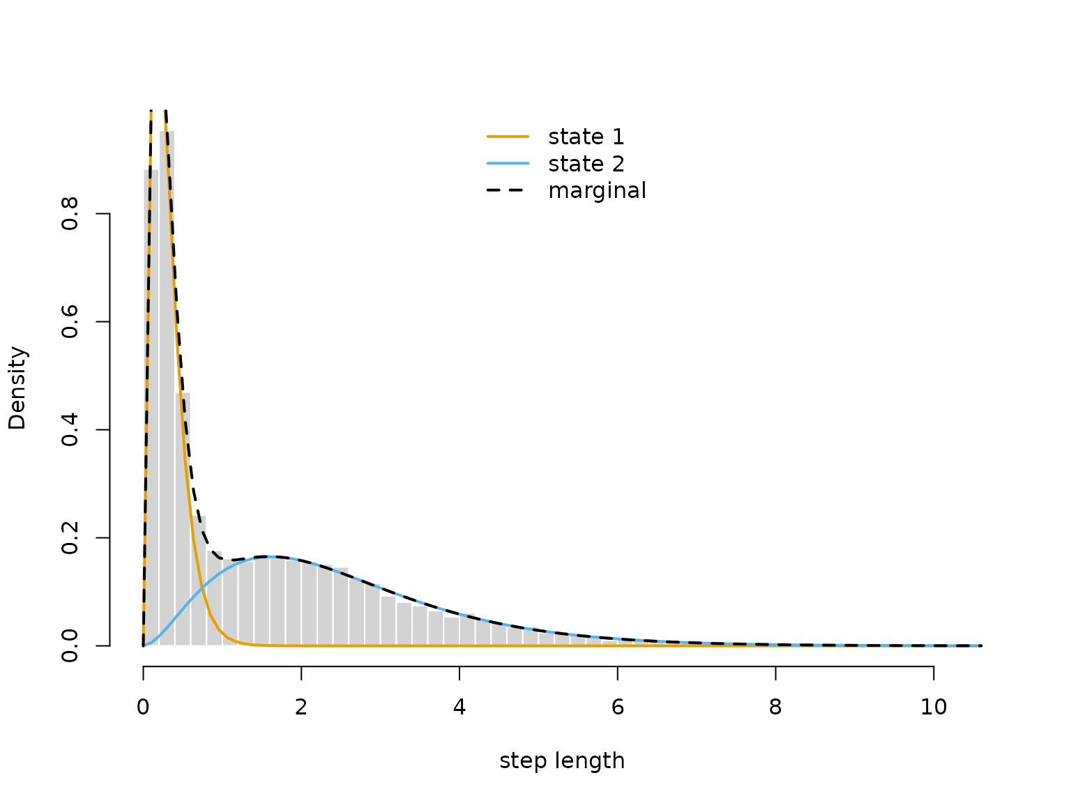

Uncertainty quantification

sdreport() gives standard errors for the unconstrained parameters and for all ADREPORT()ed quantities, the latter based on the delta method:

sdr = sdreport(obj2)
summary(sdr) # see ?summary.sdreport for more info
#>             Estimate  Std. Error
#> log_mu    -1.1923951 0.011461828
#> log_mu     0.9185717 0.009076411
#> log_sigma -1.6018327 0.016858309
#> log_sigma  0.3993241 0.013479572
#> eta       -1.6519372 0.042684391
#> eta       -1.5641927 0.041157505
#> mu         0.3034935 0.003478590
#> mu         2.5057090 0.022742845
#> sigma      0.2015268 0.003397402
#> sigma      1.4908167 0.020095571

The estimates and standard errors are also available in list format:

as.list(sdr, "Estimate") # estimated parameters
as.list(sdr, "Std")      # their standard errors
as.list(sdr, "Estimate", report = TRUE) # ADREPORT()ed quantities
as.list(sdr, "Std", report = TRUE)      # their standard errors

The delta method is not advisable for complex non-linear transformations. In this case, MCreport() draws samples of the parameters from the approximate normal distribution of the MLE, which can then be transformed by any function (see Extensions for an example).

Tips and common issues

There are some commonly occurring issues with RTMB to keep in mind. I list the main ones I have encountered here – please let me know if you encounter more so they can be added.

Non-standard distributions

If you need a non-standard probability distribution, existing implementations will likely fail due to AD incompatibility. Check whether the distribution is available in RTMBdist, which provides a library of AD-compatible distributions for use inside likelihood functions.

Operator overloading

A typical issue is that some operators may need to be overloaded to allow for automatic differentiation. In typical model setups LaMa functions handle this automatically, but if you take a more individualistic route and encounter an error like

stop("Invalid argument to 'advector' (lost class attribute?)")

you might have to overload the operator yourself. To do this put

"[<-" <- ADoverload("[<-")

as the first line of your likelihood function. If the error still prevails also add

"c" <- ADoverload("c")
"diag<-" <- ADoverload("diag<-")

which should hopefully fix the error.

Initialising with `NA`

A common problem occurs when initialising objects with NA values and then filling them with numeric values. NA is logical, which causes type mismatches that break automatic differentiation. Always initialise with numeric or NaN values instead. For example, avoid

X = array(dim = c(1,2,3))
# which is the same as
X = array(NA, dim = c(1,2,3))

and use

X = array(NaN, dim = c(1,2,3))
# or
X = array(0, dim = c(1,2,3))

Wrapping arrays in `AD()`

If you create an array and fill it with something parameter-dependent, wrap it in AD():

X <- AD(array(...))

This ensures X is an AD object from the start and that classes are compatible. Wrapping in AD() is generally a good idea to resolve the above error, as it introduces no meaningful overhead when not needed.

No `if` statements on parameters

You cannot use if statements on parameters directly, as these are not differentiable. RTMB builds the tape (computational graph) at the initial parameter value, so if branches depending on a parameter will produce gradients that are wrong elsewhere. RTMB will fail, likely without a helpful error message. if statements that do not involve parameters are typically fine, since the branch is fixed throughout optimisation.

Byte compiler side effects

Some unfortunate side effects of R’s byte compiler (enabled by default) can interfere with RTMB. If you encounter an error not covered above, try disabling it with

compiler::enableJIT(0)
#> [1] 3

References

Zucchini, Walter, Iain L. MacDonald, and Roland Langrock. 2016. Hidden Markov Models for Time Series: An Introduction Using R. Boca Raton: Chapman & Hall/CRC.

Jan-Ole Fischer

The HMM likelihood

Fitting an HMM without automatic differentiation

Generating data from a 2-state HMM

Inference by direct numerical maximum likelihood estimation

Visualising results

Writing everything yourself with RTMB

Downstream functions

Uncertainty quantification

Tips and common issues

Non-standard distributions

Operator overloading

Initialising with `NA`

Wrapping arrays in `AD()`

No `if` statements on parameters

Byte compiler side effects

Further reading

References

2 Finer control

Jan-Ole Fischer

The HMM likelihood

Fitting an HMM without automatic differentiation

Generating data from a 2-state HMM

Inference by direct numerical maximum likelihood estimation

Visualising results

Writing everything yourself with RTMB

Downstream functions

Uncertainty quantification

Tips and common issues

Non-standard distributions

Operator overloading

Initialising with NA

Wrapping arrays in AD()

No if statements on parameters

Byte compiler side effects

Further reading

References

Initialising with `NA`

Wrapping arrays in `AD()`

No `if` statements on parameters